Support Vector Machine (SVM) Classification in Python

I am going to implement a Support Vector Machine (SVM) algorithm for classification in this tutorial. I am going to visualize the data set, find the best hyperparameters to use, train a model and evalute the results. Support Vector Machine is a fast algorithm that can be used to classify data sets with linear separation, it can be helpful in text categorization.

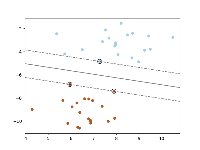
Support Vector Machine can be used for binary classification problems and for multi-class problems. Support Vector Machine is a linear method and it does not work well for data sets that have a non-linear structure (a spiral for example). Support Vector Machine can work on non-linear data by using the kernel trick. The Support Vector Machine algorithm tries do construct centered hyperplanes between classes, it wants to find hyperplanes that has the highest margin between groups of data points. The data points closest to the hyperplane are called support vectors.

The Support Vector Machine algorithm is easy to use, it is fast and the resulting model does not take up a lot of space on disk. Scikit-learn has three models for SVM that differs in their implementaion : SVC, NuSVC and LinearSVC. SVC is based on libsvm, the fit time scales at least quadratically with the number of samples. NuSVC, is similar to SVC but uses a parameter to control the number of support vectors. LinearSVC is similar to SVC, but it uses a linear kernel and are implemented in terms of liblinear rather than libsvm. I am going to use LinearSVC as it scales better to large numbers of samples.

Data set and libraries

I am going to use the Iris data set (download it) in this tutorial. The Iris data set consists of 150 flowers, each flower has four input values and one target value. I am also using the following libraries: pandas, joblib, numpy, matplotlib and scikit-learn.

Python module

I have included all code in one file, a project normally consists of many files (modules). You can create namespaces by placing files in folders and import a file by its namespaces plus its file name. A file named common.py in a annytab/learn folder is imported as import annytab.learn.common. I am going to explain more about the code in sections below.

# Import libraries
import pandas
import joblib
import numpy as np
import matplotlib.pyplot as plt
import sklearn.model_selection
import sklearn.svm
import sklearn.metrics
import sklearn.pipeline

# Visualize data set
def visualize_dataset(ds):
    
    # Print first 5 rows in data set
    print('--- First 5 rows ---\n')
    print(ds.head())

    # Print the shape
    print('\n--- Shape of data set ---\n')
    print(ds.shape)

    # Print class distribution
    print('\n--- Class distribution ---\n')
    print(ds.groupby('species').size())

    # Box plots
    plt.figure(figsize = (12, 8))
    ds.boxplot()
    #plt.show()
    plt.savefig('plots\\iris-boxplots.png')
    plt.close()

    # Scatter plots (4 subplots in 1 figure)
    figure = plt.figure(figsize = (12, 8))
    grouped_dataset = ds.groupby('species')
    values = ['sepal_length', 'sepal_width', 'petal_length', 'petal_width']
    for i, value in enumerate(values):
        plt.subplot(2, 2, i + 1) # 2 rows and 2 columns
        for name, group in grouped_dataset:
            plt.scatter(group.index, ds[value][group.index], label=name)
        plt.ylabel(value)
        plt.xlabel('index')
        plt.legend()
    #plt.show()
    plt.savefig('plots\\iris-scatterplots.png')
    
# Train and evaluate
def train_and_evaluate(X, Y):
    
    # Create a model
    model = sklearn.svm.LinearSVC(penalty='l1', loss='squared_hinge', dual=False, tol=0.0001, C=0.4, multi_class='ovr', 
                                  fit_intercept=True, intercept_scaling=1, class_weight=None, verbose=0, random_state=None, max_iter=10000)

    # Train the model on the whole data set
    model.fit(X, Y)

    # Save the model (Make sure that the folder exists)
    joblib.dump(model, 'models\\svm.jbl')

    # Evaluate on training data
    print('\n-- Training data --\n')
    predictions = model.predict(X)
    accuracy = sklearn.metrics.accuracy_score(Y, predictions)
    print('Accuracy: {0:.2f}'.format(accuracy * 100.0))
    print('Classification Report:')
    print(sklearn.metrics.classification_report(Y, predictions))
    print('Confusion Matrix:')
    print(sklearn.metrics.confusion_matrix(Y, predictions))
    print('')
    # Evaluate with 10-fold CV
    print('\n-- 10-fold CV --\n')
    predictions = sklearn.model_selection.cross_val_predict(model, X, Y, cv=10)
    accuracy = sklearn.metrics.accuracy_score(Y, predictions)
    print('Accuracy: {0:.2f}'.format(accuracy * 100.0))
    print('Classification Report:')
    print(sklearn.metrics.classification_report(Y, predictions))
    print('Confusion Matrix:')
    print(sklearn.metrics.confusion_matrix(Y, predictions))

# Perform a grid search to find the best hyperparameters
def grid_search(X, Y):

    # Create a pipeline
    clf_pipeline = sklearn.pipeline.Pipeline([
        ('m', sklearn.svm.LinearSVC(loss='squared_hinge', tol=0.0001, multi_class='ovr', dual=False, class_weight=None, verbose=0, random_state=None, max_iter=10000))
        ])

    # Set parameters (name in pipeline + name of parameter)
    parameters = { 
        'm__penalty': ('l1', 'l2'), 
        'm__C': (0.2, 0.3, 0.4, 0.5, 0.6, 0.7, 0.8, 0.9, 1.0), 
        'm__fit_intercept': (False, True),
        'm__intercept_scaling': (0.5, 1, 2)
        }

    # Create a grid search classifier
    gs_classifier = sklearn.model_selection.GridSearchCV(clf_pipeline, parameters, cv=10, iid=False, n_jobs=2, scoring='accuracy', verbose=1)
    
    # Start a search (Warning: can take a long time if the whole dataset is used)
    gs_classifier = gs_classifier.fit(X, Y)

    # Print results
    print('---- Results ----')
    print('Best score: ' + str(gs_classifier.best_score_))
    for name in sorted(parameters.keys()):
        print('{0}: {1}'.format(name, gs_classifier.best_params_[name]))

# Predict and evaluate on test data
def predict_and_evaluate(X, Y):

    # Load the model
    model = joblib.load('models\\svm.jbl')

    # Make predictions
    predictions = model.predict(X)

    # Print results
    print('\n---- Results ----')
    for i in range(len(predictions)):
        print('Input: {0}, Predicted: {1}, Actual: {2}'.format(X[i], predictions[i], Y[i]))
    accuracy = sklearn.metrics.accuracy_score(Y, predictions)
    print('\nAccuracy: {0:.2f}'.format(accuracy * 100.0))
    print('\nClassification Report:')
    print(sklearn.metrics.classification_report(Y, predictions))
    print('Confusion Matrix:')
    print(sklearn.metrics.confusion_matrix(Y, predictions))

# The main entry point for this module
def main():

    # Load data set (includes header values)
    dataset = pandas.read_csv('files\\iris.csv')

    # Visualize data set
    visualize_dataset(dataset)

    # Slice data set in values and targets (2D-array)
    X = dataset.values[:,0:4]
    Y = dataset.values[:,4]

    # Split data set in train and test (use random state to get the same split every time, and stratify to keep balance)
    X_train, X_test, Y_train, Y_test = sklearn.model_selection.train_test_split(X, Y, test_size=0.2, random_state=1, stratify=Y)

    # Make sure that data still is balanced
    print('\n--- Class balance ---\n')
    print(np.unique(Y_train, return_counts=True))
    print(np.unique(Y_test, return_counts=True))

    # Perform a grid search
    #grid_search(X, Y)

    # Train and evaluate
    #train_and_evaluate(X_train, Y_train)

    # Predict on test set
    predict_and_evaluate(X_test, Y_test)

# Tell python to run main method
if __name__ == "__main__": main()

Load and visualize the data set

The data set is loaded with pandas by using an relative path to the root of the project, use an absolute path if your files is stored outside of the project. We want to visualize the data set to make sure that it is balanced and we want to learn more about the data. It is important to have a balanced data set when performing classification, every class will be trained equally many times with a balanced training set. We can plot a data set to find patterns, remove outliers and decide on the most suitable algorithms to use.

# Load data set (includes header values)
dataset = pandas.read_csv('files\\iris.csv')

# Visualize data set
visualize_dataset(dataset)

--- First 5 rows ---
   sepal_length  sepal_width  petal_length  petal_width      species
0           5.1          3.5           1.4          0.2  Iris-setosa
1           4.9          3.0           1.4          0.2  Iris-setosa
2           4.7          3.2           1.3          0.2  Iris-setosa
3           4.6          3.1           1.5          0.2  Iris-setosa
4           5.0          3.6           1.4          0.2  Iris-setosa

--- Shape of dataset ---
(150, 5)

--- Class distribution ---
species
Iris-setosa        50
Iris-versicolor    50
Iris-virginica     50
dtype: int64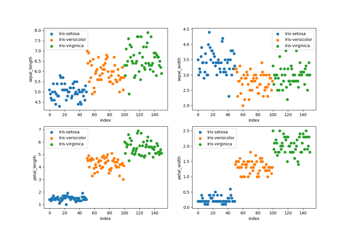

Split data set

I first need to slice values in the data set to get input values (X) and output values (Y), the first 4 columns is input values and the last column is the target value. I split the data set in a training set and a test set, 80 % is for training and 20 % for test. I want to make sure that data sets still are balanced after this split and I therefore use a stratify parameter.

# Slice data set in values and targets (2D-array)
X = dataset.values[:,0:4]
Y = dataset.values[:,4]

# Split data set in train and test (use random state to get the same split every time, and stratify to keep balance)
X_train, X_test, Y_train, Y_test = sklearn.model_selection.train_test_split(X, Y, test_size=0.2, random_state=1, stratify=Y)

# Make sure that data still is balanced
print('\n--- Class balance ---\n')
print(np.unique(Y_train, return_counts=True))
print(np.unique(Y_test, return_counts=True))

Baseline performance

Our data set has 150 flowers and 50 flowers in each class, our training set has the same balance. A random prediction will be correct in 33 % (50/150) of all cases and our model must have an accuracy that is better than 33 % to be useful.

Grid Search

I am doing a grid search to find the best hyperparameters to use for training. A grid search can take a long time to perform on large data sets but it’s probably faster than a manual process. The ouput from this process is shown below and I am going to use these parameters when I train the model.

# Perform a grid search
grid_search(X, Y)

Fitting 10 folds for each of 108 candidates, totalling 1080 fits
[Parallel(n_jobs=2)]: Using backend LokyBackend with 2 concurrent workers.
[Parallel(n_jobs=2)]: Done 968 tasks      | elapsed:    2.9s
[Parallel(n_jobs=2)]: Done 1080 out of 1080 | elapsed:    3.1s finished

---- Results ----
Best score: 0.9666666666666668
m__C: 0.4
m__fit_intercept: True
m__intercept_scaling: 1
m__penalty: l1

Training and evaluation

I am training the model by using the hyperparameters from the grid search and save the model to a file with joblib. Evaluation is made on the training set and with cross-validation. The cross-validation evaluation will give a hint on the generalization performance of the model. I had 95 % accuracy on training data and 95 % accuracy with 10-fold cross validation.

# Train and evaluate
train_and_evaluate(X_train, Y_train)

-- Training data --
Accuracy: 95.00
Classification Report:
                 precision    recall  f1-score   support

    Iris-setosa       1.00      1.00      1.00        40
Iris-versicolor       0.95      0.90      0.92        40
 Iris-virginica       0.90      0.95      0.93        40

       accuracy                           0.95       120
      macro avg       0.95      0.95      0.95       120
   weighted avg       0.95      0.95      0.95       120

Confusion Matrix:
[[40  0  0]
 [ 0 36  4]
 [ 0  2 38]]


-- 10-fold CV --
Accuracy: 95.00
Classification Report:
                 precision    recall  f1-score   support

    Iris-setosa       1.00      1.00      1.00        40
Iris-versicolor       0.93      0.93      0.93        40
 Iris-virginica       0.93      0.93      0.93        40

       accuracy                           0.95       120
      macro avg       0.95      0.95      0.95       120
   weighted avg       0.95      0.95      0.95       120

Confusion Matrix:
[[40  0  0]
 [ 0 37  3]
 [ 0  3 37]]

Test and evaluation

The final step in this process is to make predictions and evaluate the performance on the test data set. I load the model, make predictions and print the results. The X variable is a 2D array, if you want to make a prediction on one flower, then you need to set the input like this: X = np.array([[7.3, 2.9, 6.3, 1.8]]).

# Predict on test set
predict_and_evaluate(X_test, Y_test)

---- Results ----
Input: [7.3 2.9 6.3 1.8], Predicted: Iris-virginica, Actual: Iris-virginica
Input: [4.9 3.1 1.5 0.1], Predicted: Iris-setosa, Actual: Iris-setosa
Input: [5.1 2.5 3.0 1.1], Predicted: Iris-versicolor, Actual: Iris-versicolor
Input: [4.8 3.4 1.6 0.2], Predicted: Iris-setosa, Actual: Iris-setosa
Input: [5.0 3.5 1.6 0.6], Predicted: Iris-setosa, Actual: Iris-setosa
Input: [5.1 3.5 1.4 0.2], Predicted: Iris-setosa, Actual: Iris-setosa
Input: [6.2 3.4 5.4 2.3], Predicted: Iris-virginica, Actual: Iris-virginica
Input: [6.4 2.7 5.3 1.9], Predicted: Iris-virginica, Actual: Iris-virginica
Input: [5.6 2.8 4.9 2.0], Predicted: Iris-virginica, Actual: Iris-virginica
Input: [6.8 2.8 4.8 1.4], Predicted: Iris-versicolor, Actual: Iris-versicolor
Input: [5.4 3.9 1.3 0.4], Predicted: Iris-setosa, Actual: Iris-setosa
Input: [5.5 2.3 4.0 1.3], Predicted: Iris-versicolor, Actual: Iris-versicolor
Input: [6.8 3.0 5.5 2.1], Predicted: Iris-virginica, Actual: Iris-virginica
Input: [6.0 2.2 4.0 1.0], Predicted: Iris-versicolor, Actual: Iris-versicolor
Input: [5.7 2.5 5.0 2.0], Predicted: Iris-virginica, Actual: Iris-virginica
Input: [5.7 4.4 1.5 0.4], Predicted: Iris-setosa, Actual: Iris-setosa
Input: [7.1 3.0 5.9 2.1], Predicted: Iris-virginica, Actual: Iris-virginica
Input: [6.1 2.8 4.0 1.3], Predicted: Iris-versicolor, Actual: Iris-versicolor
Input: [4.9 2.4 3.3 1.0], Predicted: Iris-versicolor, Actual: Iris-versicolor
Input: [6.1 3.0 4.9 1.8], Predicted: Iris-virginica, Actual: Iris-virginica
Input: [6.4 2.9 4.3 1.3], Predicted: Iris-versicolor, Actual: Iris-versicolor
Input: [5.6 3.0 4.5 1.5], Predicted: Iris-versicolor, Actual: Iris-versicolor
Input: [4.9 3.1 1.5 0.1], Predicted: Iris-setosa, Actual: Iris-setosa
Input: [4.4 2.9 1.4 0.2], Predicted: Iris-setosa, Actual: Iris-setosa
Input: [6.5 3.0 5.2 2.0], Predicted: Iris-virginica, Actual: Iris-virginica
Input: [4.9 2.5 4.5 1.7], Predicted: Iris-virginica, Actual: Iris-virginica
Input: [5.4 3.9 1.7 0.4], Predicted: Iris-setosa, Actual: Iris-setosa
Input: [4.8 3.0 1.4 0.1], Predicted: Iris-setosa, Actual: Iris-setosa
Input: [6.3 3.3 4.7 1.6], Predicted: Iris-versicolor, Actual: Iris-versicolor
Input: [6.5 2.8 4.6 1.5], Predicted: Iris-versicolor, Actual: Iris-versicolor

Accuracy: 100.00

Classification Report:
                 precision    recall  f1-score   support

    Iris-setosa       1.00      1.00      1.00        10
Iris-versicolor       1.00      1.00      1.00        10
 Iris-virginica       1.00      1.00      1.00        10

       accuracy                           1.00        30
      macro avg       1.00      1.00      1.00        30
   weighted avg       1.00      1.00      1.00        30

Confusion Matrix:
[[10  0  0]
 [ 0 10  0]
 [ 0  0 10]]