I am going to use Multinomial Naive Bayes and Python to perform text classification in this tutorial. I am going to use the 20 Newsgroups data set, visualize the data set, preprocess the text, perform a grid search, train a model and evaluate the performance.
Naive Bayes is a group of algorithms that is used for classification in machine learning. Naive Bayes classifiers are based on Bayes theorem, a probability is calculated for each category and the category with the highest probability will be the predicted category. Gaussian Naive Bayes deals with continuous variables that are assumed to have a normal (Gaussian) distribution. Multinomial Naive Bayes deals with discrete variables that is a result from counting and Bernoulli Naive Bayes deals with boolean variables that is a result from determining an existence or not.
Multinominal Naive Bayes and Bernoulli Naive Bayes is well suited for text classification tasks. Multinomial Naive Bayes takes word count into consideration while Bernoulli Naive Bayes only takes word occurrence into consideration when we are working with text classification. Bernoulli Naive Bayes may be prefered if we do not need the added complexity that is offered by Multinomial Naive Bayes.
Data set and libraries
We are going to use the 20 Newsgroups data set (download it) in this tutorial. You shall download 20news-bydate.tar.gz, this data set is sorted by date and divided into a training set and a test set. Unpack the file to a folder (20news_bydate), files is divided into folders where the folder name represents the name of a category. You will need to have the following libraries: pandas, joblib, numpy, matplotlib, nltk and scikit-learn.
Preprocess data
I have created a common module (common.py) that includes a function to preprocess data, this function will be called from more than one module. The folder structure for this module is annytab/naive_bayes and this means that the namespace is annytab.naive_bayes. This function will process each article in the data set and remove headers, footers, quotes, punctations and digits. I am also using a stemmer to stem each word in each article, this process takes some time and you may want to comment this line to speed things up. You can use a lemmatizer instead of a stemmer if you want, you might need to download WordNetLemmatizer.
# Import libraries
import re
import string
import nltk.stem

# Download WordNetLemmatizer
# nltk.download()

# Variables
QUOTES = re.compile(r'(writes in|writes:|wrote:|says:|said:|^In article|^Quoted from|^\||^>)')

# Preprocess data
def preprocess_data(data):

    # Create a stemmer/lemmatizer
    stemmer = nltk.stem.SnowballStemmer('english')
    #lemmer = nltk.stem.WordNetLemmatizer()

    for i in range(len(data)):
        # Remove header
        _, _, data[i] = data[i].partition('\n\n')
        # Remove footer
        lines = data[i].strip().split('\n')
        for line_num in range(len(lines) - 1, -1, -1):
            line = lines[line_num]
            if line.strip().strip('-') == '':
                break
        if line_num > 0:
            data[i] = '\n'.join(lines[:line_num])
        # Remove quotes
        data[i] = '\n'.join([line for line in data[i].split('\n') if not QUOTES.search(line)])
        # Remove punctation (!"#$%&'()*+,-./:;<=>?@[\]^_`{|}~)
        data[i] = data[i].translate(str.maketrans('', '', string.punctuation))
        # Remove digits
        data[i] = re.sub('\d', '', data[i])
        # Stem words
        data[i] = ' '.join([stemmer.stem(word) for word in data[i].split()])
        #data[i] = ' '.join([lemmer.lemmatize(word) for word in data[i].split()])

    # Return data
    return data
Training module
# Import libraries
import joblib
import numpy as np
import matplotlib.pyplot as plt
import sklearn.datasets
import sklearn.feature_extraction.text
import sklearn.naive_bayes
import sklearn.metrics
import sklearn.model_selection
import sklearn.pipeline

import annytab.naive_bayes.common as common

# Visualize dataset
def visualize_dataset(ds):

    # Print dataset
    #for i in range(5):
    #    print(ds.data[i])
    #print(ds.target_names)
    print('--- Information ---')
    print('Number of articles: ' + str(len(ds.data)))
    print('Number of categories: ' + str(len(ds.target_names)))

    # Count number of articles in each category
    plot_X = np.arange(20, dtype=np.int16)
    plot_Y = np.zeros(20)
    for i in range(len(ds.data)):
        plot_Y[ds.target[i]] += 1

    print('\n--- Class distribution ---')
    for i in range(len(plot_X)):
        print('{0}: {1:.0f}'.format(ds.target_names[plot_X[i]], plot_Y[i]))

    # Plot the balance of the dataset
    figure = plt.figure(figsize = (16, 10))
    figure.suptitle('Balance of data set', fontsize=16)
    plt.bar(plot_X, plot_Y, align='center', color='rgbkymc')
    plt.xticks(plot_X, ds.target_names, rotation=25, horizontalalignment='right')
    #plt.show()
    plt.savefig('C:\\DATA\\Python-models\\accountant\\sklearn\\20-newsgroups-balance.png')

# Perform a grid search to find the best hyperparameters
def grid_search(train):

    # Create a pipeline
    clf_pipeline = sklearn.pipeline.Pipeline([
        ('v', sklearn.feature_extraction.text.CountVectorizer(strip_accents='ascii', stop_words='english')),
        ('t', sklearn.feature_extraction.text.TfidfTransformer()),
        ('c', sklearn.naive_bayes.MultinomialNB(fit_prior=True, class_prior=None))
        ])

    # Set parameters (name in pipeline + name of parameter)
    parameters = {
        'v__ngram_range': [(1, 1), (1, 2), (1, 3), (1, 4)],
        'v__lowercase': (True, False),
        't__use_idf': (True, False),
        'c__alpha': (0.3, 0.6, 1.0) }

    # Create a grid search classifier
    gs_classifier = sklearn.model_selection.GridSearchCV(clf_pipeline, parameters, cv=5, iid=False, n_jobs=2, scoring='accuracy', verbose=1)

    # Start a search (Warning: takes a long time if the whole dataset is used)
    # Slice: (train.data[:4000], train.target[:4000])
    gs_classifier = gs_classifier.fit(train.data, train.target)

    # Print results
    print('---- Results ----')
    print('Best score: ' + str(gs_classifier.best_score_))
    for name in sorted(parameters.keys()):
        print('{0}: {1}'.format(name, gs_classifier.best_params_[name]))

# Train and evaluate a model
def train_and_evaluate(train):

    # Convert to bag of words
    count_vect = sklearn.feature_extraction.text.CountVectorizer(strip_accents='ascii', stop_words='english', lowercase=True, ngram_range=(1,1))
    X = count_vect.fit_transform(train.data)

    # Convert from occurrences to frequencies
    # Occurrence count is a good start but there is an issue: longer documents will have higher average count values than shorter documents, even though they might talk about the same topics.
    # To avoid these potential discrepancies it suffices to divide the number of occurrences of each word in a document by the total number of words in the document: these new features are called tf for Term Frequencies.
    transformer = sklearn.feature_extraction.text.TfidfTransformer()
    X = transformer.fit_transform(X)

    # Create a model
    model = sklearn.naive_bayes.MultinomialNB(alpha=0.3, fit_prior=True, class_prior=None)

    # Train the model
    model.fit(X, train.target)

    # Save models
    joblib.dump(count_vect, 'C:\\DATA\\Python-models\\accountant\\sklearn\\vectorizer.jbl')
    joblib.dump(transformer, 'C:\\DATA\\Python-models\\accountant\\sklearn\\transformer.jbl')
    joblib.dump(model, 'C:\\DATA\\Python-models\\accountant\\sklearn\\model.jbl')

    # Evaluate on training data
    print('-- Training data --')
    predictions = model.predict(X)
    accuracy = sklearn.metrics.accuracy_score(train.target, predictions)
    print('Accuracy: {0:.2f}'.format(accuracy * 100.0))
    print('Classification Report:')
    print(sklearn.metrics.classification_report(train.target, predictions, target_names=train.target_names))
    print('')
    # Evaluate with 10-fold CV
    print('-- 10-fold CV --')
    predictions = sklearn.model_selection.cross_val_predict(model, X, train.target, cv=10)
    accuracy = sklearn.metrics.accuracy_score(train.target, predictions)
    print('Accuracy: {0:.2f}'.format(accuracy * 100.0))
    print('Classification Report:')
    print(sklearn.metrics.classification_report(train.target, predictions, target_names=train.target_names))

# The main entry point for this module
def main():

    # Load train dataset
    # Load text files with categories as subfolder names
    # Individual samples are assumed to be files stored a two levels folder structure
    # The folder names are used as supervised signal label names. The individual file names are not important.
    train = sklearn.datasets.load_files('C:\\DATA\\Python-models\\20news_bydate\\20news-bydate-train', shuffle=False, load_content=True, encoding='latin1')

    # Visualize dataset
    #visualize_dataset(train)

    # Preprocess data
    train.data = common.preprocess_data(train.data)

    # Print cleaned data
    #print(train.data[0])

    # Grid search
    #grid_search(train)

    # Train and evaluate
    train_and_evaluate(train)

# Tell python to run main method
if __name__ == "__main__": main()
Evaluation module
# Import libraries
import joblib
import numpy as np
import sklearn.datasets
import sklearn.feature_extraction.text
import sklearn.naive_bayes
import sklearn.metrics

import annytab.naive_bayes.common as common

# Test and evaluate a model
def test_and_evaluate(test):

    # Load models
    vectorizer = joblib.load('C:\\DATA\\Python-models\\accountant\\sklearn\\vectorizer.jbl')
    transformer = joblib.load('C:\\DATA\\Python-models\\accountant\\sklearn\\transformer.jbl')
    model = joblib.load('C:\\DATA\\Python-models\\accountant\\sklearn\\model.jbl')

    # Convert to bag of words
    X = vectorizer.transform(test.data)

    # Convert from occurrences to frequencies
    X = transformer.transform(X)

    # Make predictions
    predictions = model.predict(X)

    # Print results
    print('-- Results --')
    accuracy = sklearn.metrics.accuracy_score(test.target, predictions)
    print('Accuracy: {0:.2f}'.format(accuracy * 100.0))
    print('Classification Report:')
    print(sklearn.metrics.classification_report(test.target, predictions, target_names=test.target_names))

# The main entry point for this module
def main():

    # Load test dataset
    # Load text files with categories as subfolder names
    # Individual samples are assumed to be files stored a two levels folder structure
    # The folder names are used as supervised signal label names. The individual file names are not important.
    test = sklearn.datasets.load_files('C:\\DATA\\Python-models\\20news_bydate\\20news-bydate-test', shuffle=False, load_content=True, encoding='latin1')

    # Preprocess data
    test.data = common.preprocess_data(test.data)

    # Test and evaluate
    test_and_evaluate(test)

# Tell python to run main method
if __name__ == "__main__": main()
Visualize data set
The code to visualize the data set is included in the training module. We mainly want to see the balance of the training set, a balanced data set is important in classification algorithms. The data set is not perfectly balanced, the most frequent category (rec.sport.hockey) have 600 articles and the least frequent category (talk.religion.misc) have 377 articles. The probability of correctly predicting the most frequent category at random is 5.3 % (600 *100/11314), our model needs to have a higher probability than this to be useful.
# Load train data set
train = sklearn.datasets.load_files('C:\\DATA\\Python-models\\20news_bydate\\20news-bydate-train', shuffle=False, load_content=True, encoding='latin1')

# Visualize data set
visualize_dataset(train)

--- Information ---
Number of articles: 11314
Number of categories: 20

--- Class distribution ---
alt.atheism: 480
comp.graphics: 584
comp.os.ms-windows.misc: 591
comp.sys.ibm.pc.hardware: 590
comp.sys.mac.hardware: 578
comp.windows.x: 593
misc.forsale: 585
rec.autos: 594
rec.motorcycles: 598
rec.sport.baseball: 597
rec.sport.hockey: 600
sci.crypt: 595
sci.electronics: 591
sci.med: 594
sci.space: 593
soc.religion.christian: 599
talk.politics.guns: 546
talk.politics.mideast: 564
talk.politics.misc: 465
talk.religion.misc: 377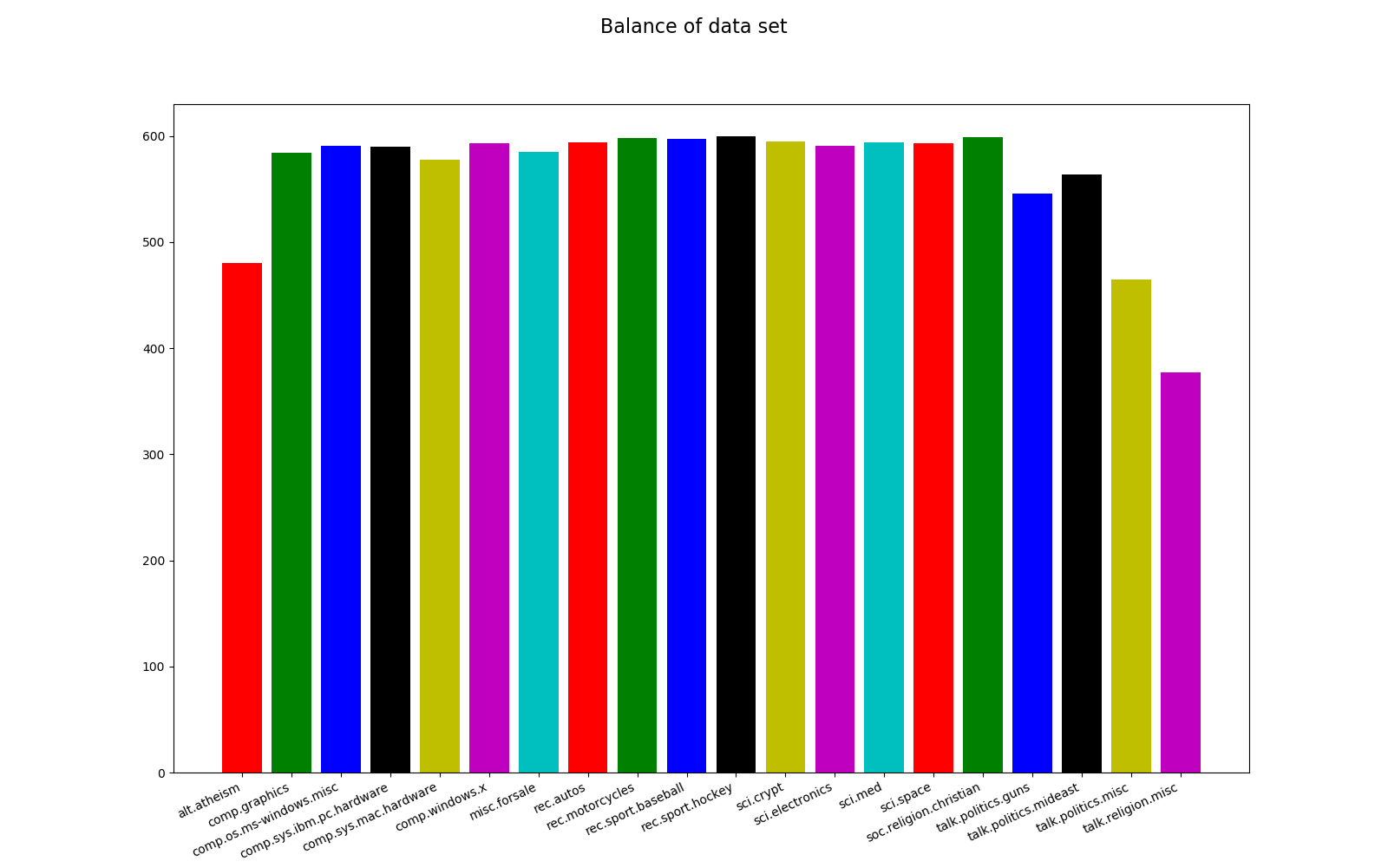
Grid Search
I am doing a grid search to find the best parameters to use for training. A grid search can take a long time to perform on large data sets and you can therefore slice the data set and perform the grid search on a smaller set. The ouput from this process is shown below and I am going to use these parameters when I train the model.
Fitting 5 folds for each of 48 candidates, totalling 240 fits
[Parallel(n_jobs=2)]: Using backend LokyBackend with 2 concurrent workers.
[Parallel(n_jobs=2)]: Done  46 tasks      | elapsed:  2.2min
[Parallel(n_jobs=2)]: Done 196 tasks      | elapsed: 10.2min
[Parallel(n_jobs=2)]: Done 240 out of 240 | elapsed: 12.6min finished
---- Results ----
Best score: 0.7087874275996338
c__alpha: 0.3
t__use_idf: True
v__lowercase: True
v__ngram_range: (1, 1)
Train and evaluate
I am loading files from the 20news-bydate-train folder, I preprocess each file and train the model by using the parameters from the grid search, models is saved to files with joblib. Evaluation is made on the training set and with cross-validation. The cross-validation evaluation will give a hint on the generalization performance of the model. I had 89.37 % accuracy on training data and 71.66 % accuracy with 10-fold cross validation.
# Load train dataset
train = sklearn.datasets.load_files('C:\\DATA\\Python-models\\20news_bydate\\20news-bydate-train', shuffle=False, load_content=True, encoding='latin1')

# Preprocess data
train.data = common.preprocess_data(train.data)

# Train and evaluate
train_and_evaluate(train)

-- Training data --
Accuracy: 89.37
Classification Report:
                          precision    recall  f1-score   support

             alt.atheism       0.95      0.74      0.83       480
           comp.graphics       0.93      0.89      0.91       584
 comp.os.ms-windows.misc       0.92      0.87      0.89       591
comp.sys.ibm.pc.hardware       0.83      0.93      0.88       590
   comp.sys.mac.hardware       0.96      0.89      0.92       578
          comp.windows.x       0.94      0.96      0.95       593
            misc.forsale       0.96      0.88      0.91       585
               rec.autos       0.95      0.88      0.92       594
         rec.motorcycles       0.98      0.93      0.96       598
      rec.sport.baseball       0.99      0.93      0.96       597
        rec.sport.hockey       0.65      0.97      0.78       600
               sci.crypt       0.90      0.95      0.92       595
         sci.electronics       0.95      0.89      0.92       591
                 sci.med       0.98      0.95      0.96       594
               sci.space       0.97      0.95      0.96       593
  soc.religion.christian       0.64      0.98      0.77       599
      talk.politics.guns       0.88      0.95      0.91       546
   talk.politics.mideast       0.94      0.94      0.94       564
      talk.politics.misc       0.98      0.86      0.91       465
      talk.religion.misc       1.00      0.30      0.46       377

                accuracy                           0.89     11314
               macro avg       0.92      0.88      0.88     11314
            weighted avg       0.91      0.89      0.89     11314


-- 10-fold CV --
Accuracy: 71.66
Classification Report:
                          precision    recall  f1-score   support

             alt.atheism       0.81      0.33      0.47       480
           comp.graphics       0.72      0.66      0.69       584
 comp.os.ms-windows.misc       0.74      0.60      0.66       591
comp.sys.ibm.pc.hardware       0.61      0.74      0.67       590
   comp.sys.mac.hardware       0.78      0.71      0.75       578
          comp.windows.x       0.80      0.85      0.82       593
            misc.forsale       0.82      0.67      0.73       585
               rec.autos       0.81      0.72      0.76       594
         rec.motorcycles       0.81      0.73      0.77       598
      rec.sport.baseball       0.91      0.81      0.86       597
        rec.sport.hockey       0.59      0.90      0.71       600
               sci.crypt       0.64      0.87      0.74       595
         sci.electronics       0.78      0.69      0.73       591
                 sci.med       0.88      0.82      0.85       594
               sci.space       0.83      0.78      0.80       593
  soc.religion.christian       0.43      0.94      0.59       599
      talk.politics.guns       0.68      0.81      0.74       546
   talk.politics.mideast       0.81      0.82      0.81       564
      talk.politics.misc       0.86      0.49      0.63       465
      talk.religion.misc       0.58      0.04      0.07       377

                accuracy                           0.72     11314
               macro avg       0.74      0.70      0.69     11314
            weighted avg       0.75      0.72      0.71     11314
Test and evaluate
Testing and evaluation is performed in the evaluation module. I am loading files from the 20news-bydate-test folder, I preprocess the test data, I load models and I evaluate the performance. I am loading 3 models, a CountVectorizer, a TfidfTransformer and a MultinomialNB model. The output from the evaluation is shown below.
# Load test dataset
test = sklearn.datasets.load_files('C:\\DATA\\Python-models\\20news_bydate\\20news-bydate-test', shuffle=False, load_content=True, encoding='latin1')

# Preprocess data
test.data = common.preprocess_data(test.data)

# Print cleaned data
print(test.data[0])

# Test and evaluate
test_and_evaluate(test)

-- Results --
Accuracy: 67.83
Classification Report:
                          precision    recall  f1-score   support

             alt.atheism       0.75      0.24      0.36       319
           comp.graphics       0.66      0.66      0.66       389
 comp.os.ms-windows.misc       0.72      0.54      0.62       394
comp.sys.ibm.pc.hardware       0.59      0.72      0.65       392
   comp.sys.mac.hardware       0.75      0.68      0.71       385
          comp.windows.x       0.80      0.76      0.78       395
            misc.forsale       0.82      0.68      0.74       390
               rec.autos       0.83      0.74      0.78       396
         rec.motorcycles       0.83      0.73      0.78       398
      rec.sport.baseball       0.94      0.81      0.87       397
        rec.sport.hockey       0.59      0.94      0.72       399
               sci.crypt       0.60      0.80      0.69       396
         sci.electronics       0.69      0.55      0.61       393
                 sci.med       0.86      0.78      0.82       396
               sci.space       0.76      0.77      0.77       394
  soc.religion.christian       0.39      0.92      0.55       398
      talk.politics.guns       0.54      0.72      0.62       364
   talk.politics.mideast       0.80      0.80      0.80       376
      talk.politics.misc       0.80      0.34      0.48       310
      talk.religion.misc       0.75      0.01      0.02       251

                accuracy                           0.68      7532
               macro avg       0.72      0.66      0.65      7532
            weighted avg       0.72      0.68      0.67      7532