This tutorial shows you how to implement a linear regression algorithm to predict share prices in Python. I am using data from Ericsson AB to predict the share price of ericsson. I am going to prepare data, visualize data, train a model, evaluate the model and use the model to make predictions.
Stock prices reflects expectations about the ability to generate cash flows and earnings in the future. Earnings are more stable than cash flows, but earnings is influenced by applied accounting standards and cash flows is not. My theory is that the share prices is affected by revenue, earnings, equity, free cash flow, changes in revenue, changes in earnings, changes in free cash flow and the interest rate. The interest rate is an alternative to investments in stocks and it affects the required rate of return. I am going to use market value (share price * number of shares) as the target value to make input data independent of the actual number of shares.
Share prices is affected by dividend payouts, a share price usually drops with an amount that corresponds to the dividend per share on the payout day. I have adjusted free cash flows for new share issues and dividend payouts. Earnings has not been adjusted for dividends but equity is affected by dividend payouts as equity decreases when there has been dividend payouts.
Stock prices is mainly influenced by expectations about the future and I will take this into consideration by using annual revenues, annual earnings and annual free cash flows from the first day in the year. My input data will have daily changes in market value and interest rate but only annual changes in revenue, earnings, free cash flow, equity, growth in revenue, growth in earnings and growth in free cash flows. Growth is measured as the difference between the revenue, earnings or free cash flows during a year compared to the previous year. It is impossible to use percentage changes as earnings can be both negative and positive.
Stock prices move up and down in a short perspective but they tend to move to an average price over time (Mean reversion). A linear regression model deals with mean values as regression means that values will return to a mean. Linear regression models a relationship between a dependent variable (Y) and one or more inpendent variables (X). A linear regression model wants to find a function that best fits the input data.
Data set and libraries
I am going to use a data set (download it) with information about Ericsson AB in this tutorial. Ericsson AB was founded in 1918 and has had periods of high growth, periods of stagnation and periods of declination. This data set contains data from 1987 to 2018, it has one dependent variable (market value) and 8 independent variables. You will need the following libraries for this tutorial: numpy, pandas, matplotlib, statsmodels, scikit-learn and joblib.
Common module
I have a common module (common.py) that includes one method. The folder structure for this module is annytab/stock_prediction and this means that the namespace is annytab.stock_prediction. All other modules is stored in the same folder.
# Remove outliers from a data set
def remove_outliers(ds, col_name):
    q1 = ds[col_name].quantile(0.25)
    q3 = ds[col_name].quantile(0.75)
    iqr = q3-q1 #Interquartile range
    fence_low  = q1-1.5*iqr
    fence_high = q3+1.5*iqr
    ds = ds.loc[(ds[col_name] > fence_low) & (ds[col_name] < fence_high)]
    return ds
Prepare data
We have a module that is dedicated for data preparation and data visualization. The contents of this file is shown below.
# Import libraries
import numpy as np
import pandas as pd
import matplotlib.pyplot as plt
import statsmodels.api as sm

import annytab.stock_prediction.common as common

# Visualize the dataset
def visualize(ds):

    # Count the number columns
    count = len(ds.columns.values)

    # Print number of columns
    print('--- Columns ---\n')
    print(count)

    # Get data labels (all labels except the target label)
    data_labels = list(ds.columns.values[1:count])
    ols_labels = data_labels.copy()
    ols_labels.insert(0, 'CONSTANT')

    # Print first 5 rows in data set
    print('\n--- First 5 rows ---\n')
    print(ds.head())

    # Print the shape
    print('\n--- Shape of data set ---\n')
    print(ds.shape)

    # Print labels
    print('\n--- Data labels ---\n')
    print(data_labels)

    # Plot Y in a line diagram
    figure = plt.figure(figsize = (12, 8))
    figure.suptitle('ERICSSON B', fontsize=16)
    plt.plot(ds['MARKET VALUE'])
    plt.ylabel('MARKET VALUE')
    plt.xlabel('INDICES')
    #plt.show() # Show or save the plot (can not do both)
    plt.savefig('plots\\ericsson-chart.png')
    plt.close()

    # Scatter plots (8 subplots in 1 figure)
    figure = plt.figure(figsize = (12, 8))
    figure.suptitle('CORRELATION WITH MARKET VALUE', fontsize=16)
    plt.subplots_adjust(top = 0.9, bottom=0.1, hspace=0.5, wspace=0.2)
    for i, value in enumerate(data_labels):
            plt.subplot(2, 4, i + 1) # 2 rows and 4 columns
            plt.scatter(ds[value], ds['MARKET VALUE'])
            plt.title(value)
    #plt.show() # Show or save the plot (can not do both)
    plt.savefig('plots\\ericsson-scatterplots.png')
    plt.close()

    # Slice data set in data (X) and target (Y)
    X = dataset.values[:,1:count] # DATA
    Y = dataset.values[:,0] # MARKET VALUE

    # Output OLS-statistics
    X = sm.add_constant(X)
    model = sm.OLS(Y, X)
    model.data.ynames = 'MARKET VALUE'
    model.data.xnames = ols_labels
    results = model.fit()
    f = open('plots\\ericsson-summary.txt', 'w')
    f.write(str(results.summary()))
    f.close()

# Load data set
dataset = pd.read_csv('files\\ericsson.csv', sep=';')

# Remove outliers
#dataset = common.remove_outliers(dataset, 'MARKET VALUE')

# Remove E-CHANGE and FCF-CHANGE
#dataset = dataset.drop(columns=['E-CHANGE', 'FCF-CHANGE'])

# Visualize data set
visualize(dataset)
Load data set and visualize data
The data set is loaded with pandas by using an relative path to the root of the project, use an absolute path if your files is stored outside of the project. We are going to print information about the data set and create plots to learn more about the data set.

The market value is calculated as the share price multiplied by the total number of shares at the end of 2018. The share price of Ericsson had a strong rise and fall during the period between the end of 1999 and the beginning of 2001. This was during the dot-com bubble, it was a period of excessive speculation and many tech-companies had overvalued stock prices. We might need to remove outliers in our data set to be able to get better predictions.
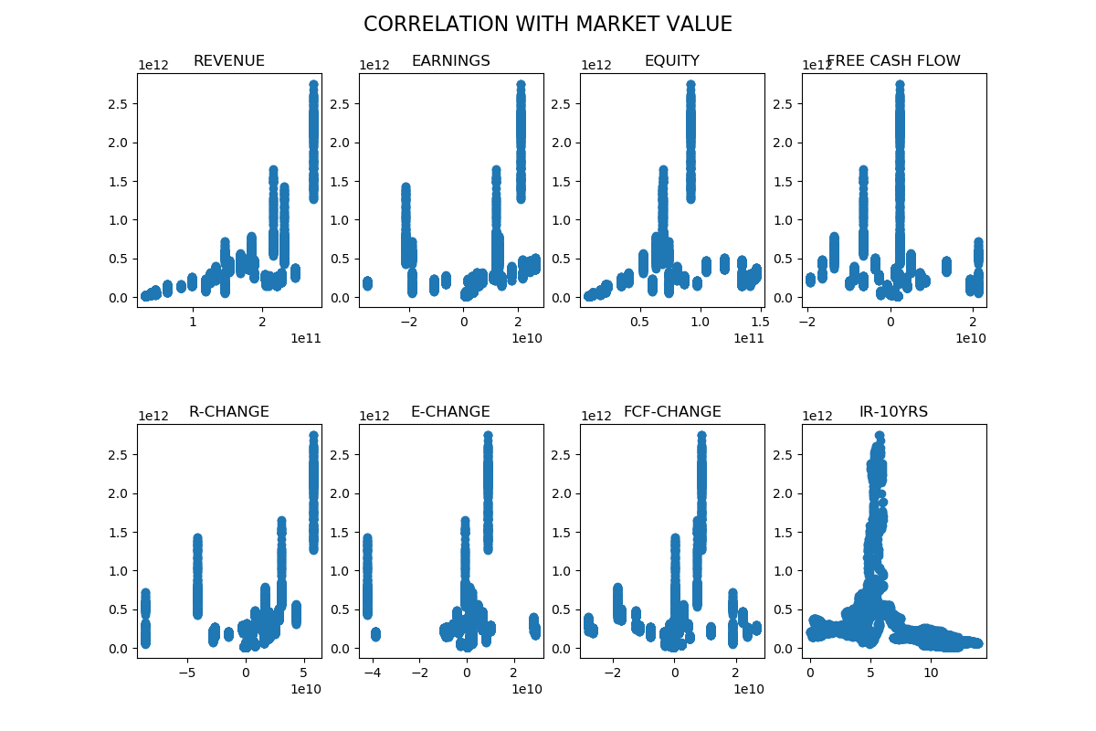
Each independent variable is plotted against the market value to get a visual picture of the correlation between each independent variable and the market value. The correlation seems to be best between revenue and market value.
                            OLS Regression Results
==============================================================================
Dep. Variable:           MARKET VALUE   R-squared:                       0.709
Model:                            OLS   Adj. R-squared:                  0.709
Method:                 Least Squares   F-statistic:                     2446.
Date:                Mon, 25 Nov 2019   Prob (F-statistic):               0.00
Time:                        10:29:00   Log-Likelihood:            -2.2056e+05
No. Observations:                8035   AIC:                         4.411e+05
Df Residuals:                    8026   BIC:                         4.412e+05
Df Model:                           8
Covariance Type:            nonrobust
==================================================================================
                     coef    std err          t      P>|t|      [0.025      0.975]
----------------------------------------------------------------------------------
CONSTANT       -6.663e+11   2.32e+10    -28.669      0.000   -7.12e+11   -6.21e+11
REVENUE            8.9168      0.078    113.885      0.000       8.763       9.070
EARNINGS          13.1772      0.380     34.645      0.000      12.432      13.923
EQUITY            -8.3278      0.142    -58.667      0.000      -8.606      -8.050
FREE CASH FLOW     1.9080      0.424      4.502      0.000       1.077       2.739
R-CHANGE          -1.9292      0.148    -13.025      0.000      -2.220      -1.639
E-CHANGE          -0.4610      0.253     -1.825      0.068      -0.956       0.034
FCF-CHANGE        -0.0176      0.275     -0.064      0.949      -0.556       0.521
IR-10YRS         3.67e+10   1.85e+09     19.861      0.000    3.31e+10    4.03e+10
==============================================================================
Omnibus:                     3545.022   Durbin-Watson:                   0.012
Prob(Omnibus):                  0.000   Jarque-Bera (JB):            25831.027
Skew:                           1.966   Prob(JB):                         0.00
Kurtosis:                      10.855   Cond. No.                     2.03e+12
==============================================================================

Warnings:
[1] Standard Errors assume that the covariance matrix of the errors is correctly specified.
[2] The condition number is large, 2.03e+12. This might indicate that there are
strong multicollinearity or other numerical problems.
I have used a OLS-model from statsmodels to get a nice statistical summary of a linear regression. The Coefficient Of Determination (r-squared) is 70.9 % and the F-statistic is 2446, this means that the model is significant. E-CHANGE and FCF-CHANGE is not significant in a t-test, the probability to get a higher t-value is to high. I have decided to remove E-CHANGE and FCF-CHANGE from the data set, I am also going to remove outliers in the data set.
Training and evaluation
The data set is loaded and sliced in data (X) and target (Y). We split the data set in a training set and a test set with a 80/20-ratio, 80 % for training and 20 % for test. I have performed a grid search and use the information from this process to set parameters in the model.
# Import libraries
import numpy as np
import pandas as pd
import sklearn
import sklearn.linear_model
import sklearn.metrics
import sklearn.pipeline
import joblib
import matplotlib.pyplot as plt

import annytab.stock_prediction.common as common

# Variables
number_of_shares = 3334151735

# Perform a grid search to find the best parameters
def grid_search(X, Y):

    # Create a pipeline
    clf_pipeline = sklearn.pipeline.Pipeline([
        ('m', sklearn.linear_model.LinearRegression(copy_X=True, n_jobs=2))
        ])

    # Set parameters (name in pipeline + name of parameter)
    parameters = {
        'm__fit_intercept': (True, False),
        'm__normalize': (True, False)
        }

    # Create a grid search classifier
    #print(sklearn.metrics.SCORERS.keys())
    gs_classifier = sklearn.model_selection.GridSearchCV(clf_pipeline, parameters, cv=10, iid=False, n_jobs=2, scoring='neg_mean_squared_error', verbose=1)

    # Start a search (Warning: can take a long time if the whole dataset is used)
    gs_classifier = gs_classifier.fit(X, Y)

    # Print results
    print('---- Results ----')
    print('Best score: ' + str(gs_classifier.best_score_))
    for name in sorted(parameters.keys()):
        print('{0}: {1}'.format(name, gs_classifier.best_params_[name]))

# Train and evaluate
def train_and_evaluate(X, Y):

    # Create a model
    model = sklearn.linear_model.LinearRegression(copy_X=True, fit_intercept=True, normalize=False, n_jobs=2)

    # Train the model
    model.fit(X, Y)

    # Save the model (Make sure that the folder exists)
    joblib.dump(model, 'models\\linear_regression.jbl')

    # Evaluate on training data
    print('\n-- Training data --\n')
    predictions = model.predict(X)
    print('r2 (coefficient of determination): {0:.2f}'.format(sklearn.metrics.r2_score(Y, predictions)))
    print('RMSE: {0:.2f}'.format(np.sqrt(sklearn.metrics.mean_squared_error(Y, predictions))))
    print('')
    # Evaluate with 10-fold CV
    print('\n-- 10-fold CV --\n')
    predictions = sklearn.model_selection.cross_val_predict(model, X, Y, cv=10)
    print('r2 (coefficient of determination): {0:.2f}'.format(sklearn.metrics.r2_score(Y, predictions)))
    print('RMSE: {0:.2f}'.format(np.sqrt(sklearn.metrics.mean_squared_error(Y, predictions))))

# Test and evaluate
def test_and_evaluate(X, Y):

    # Load the model
    model = joblib.load('models\\linear_regression.jbl')

    # Make predictions
    predictions = model.predict(X)

    # Print results
    print('\n---- Results ----')
    for i in range(len(predictions)):
        print('Predicted: {0:.2f}, Actual: {1:.2f}'.format(predictions[i] / number_of_shares, Y[i] / number_of_shares))
    print('r2 (coefficient of determination): {0:.2f}'.format(sklearn.metrics.r2_score(Y, predictions)))
    rmse = np.sqrt(sklearn.metrics.mean_squared_error(Y, predictions))
    print('RMSE: {0:.2f}'.format(rmse))
    print('RMSE / share: {0:.2f}'.format(rmse / number_of_shares))

# Make predictions
def predict(X):

    # Load the model
    model = joblib.load('models\\linear_regression.jbl')

    # Make predictions
    predictions = model.predict(X)

    # Print results
    print('\n---- Results ----')
    for i in range(len(predictions)):
        print('Input: {0}, Predicted: {1:.2f}'.format(X[i], predictions[i] / number_of_shares))

    # Plot predictions
    prices = predictions / number_of_shares
    figure = plt.figure(figsize = (12, 8))
    figure.suptitle('FUTURE PRICE PREDICTIONS', fontsize=16)
    plt.plot(prices + 1.96 * 25.74, color='red')
    plt.plot(prices - 1.96 * 25.74, color='red')
    plt.plot(['2019', '2020', '2021'], prices)
    plt.xlabel('Years')
    plt.savefig('plots\\ericsson-predictions.png')

# The main entry point for this module
def main():

    # Load data set
    ds = pd.read_csv('files\\ericsson.csv', sep=';')

    # Remove outliers
    ds = common.remove_outliers(ds, 'MARKET VALUE')

    # Remove E-CHANGE and FCF-CHANGE
    ds = ds.drop(columns=['E-CHANGE', 'FCF-CHANGE'])

    # Count the number columns
    count = len(ds.columns.values)

    # Get data labels (all labels except the target label)
    data_labels = list(ds.columns.values[1:count])

    # Slice data set in data (X) and target (Y)
    X = ds.values[:,1:count] # DATA
    Y = ds.values[:,0] # MARKET VALUE

    # Split data set in train and test (use random state to get the same split every time)
    X_train, X_test, Y_train, Y_test = sklearn.model_selection.train_test_split(X, Y, test_size=0.2, random_state=2)

    # Perform a grid search
    #grid_search(X_train, Y_train)

    # Train and evaluate
    train_and_evaluate(X_train, Y_train)

    # Test and evaluate
    #test_and_evaluate(X_test, Y_test)

    # Predict on estimates [REVENUE, EARNINGS, EQUITY, FREE CASH FLOW, R-CHANGE, IR
    #estimates = [[226852000000.000, 2892000000.000, 85935700952.700, -3698055738.150, 16014000000.000, 0.500],
    #             [236050000000.000, 16239000000.000, 96740033624.650, 11131283567.850, 9198000000.000, 0.500],
    #             [242666000000.000, 19144000000.000, 108715607394.400, 13377256804.450, 6616000000.000, 0.500]]
    #predict(estimates)

# Tell python to run main method
if __name__ == "__main__": main()
Output from grid search and evaluation
Fitting 10 folds for each of 4 candidates, totalling 40 fits
[Parallel(n_jobs=2)]: Using backend LokyBackend with 2 concurrent workers.
[Parallel(n_jobs=2)]: Done  40 out of  40 | elapsed:    0.8s finished
---- Results ----
Best score: -6.932311663824655e+21
m__fit_intercept: True
m__normalize: False
-- Training data --
r2 (coefficient of determination): 0.71
RMSE: 83107645234.47
-- 10-fold CV --
r2 (coefficient of determination): 0.71
RMSE: 83260504825.67Test and evaluate
The trained and saved model is evaluated on the test set. I load the saved model and evaluate the model on r-square and RMSE. The market value is divided by the total number of shares at the end of 2018.
Predicted: 111.80, Actual: 113.10
Predicted: 21.13, Actual: 20.18
Predicted: 17.38, Actual: 4.52
Predicted: 95.71, Actual: 75.90
Predicted: 35.90, Actual: 38.53
Predicted: 142.09, Actual: 133.97
Predicted: 69.47, Actual: 63.20
Predicted: 80.97, Actual: 59.65
Predicted: 121.41, Actual: 113.98
Predicted: 68.39, Actual: 85.55
Predicted: 20.06, Actual: 8.59
Predicted: 19.87, Actual: 10.07
Predicted: 22.12, Actual: 63.60
Predicted: 68.54, Actual: 69.80
Predicted: 64.61, Actual: 74.00
Predicted: 22.69, Actual: 19.16
Predicted: 33.87, Actual: 35.61
Predicted: 111.21, Actual: 86.75
Predicted: 83.96, Actual: 104.50
Predicted: 172.00, Actual: 201.32
Predicted: 101.12, Actual: 137.50
Predicted: 101.50, Actual: 138.50
Predicted: 96.09, Actual: 128.75
Predicted: 101.50, Actual: 137.50
Predicted: 100.67, Actual: 127.00
Predicted: 21.30, Actual: 18.83
Predicted: 108.88, Actual: 75.90
Predicted: 63.56, Actual: 87.90
Predicted: 122.36, Actual: 142.41
Predicted: 17.37, Actual: 17.97
Predicted: 21.32, Actual: 19.76
Predicted: 17.29, Actual: 6.80
Predicted: 105.57, Actual: 82.10
Predicted: 101.36, Actual: 134.50
Predicted: 106.22, Actual: 87.10
Predicted: 158.11, Actual: 193.19
Predicted: 67.68, Actual: 75.70
Predicted: 122.78, Actual: 132.48
Predicted: 16.24, Actual: 5.02
Predicted: 21.71, Actual: 52.50
Predicted: 62.98, Actual: 80.95
Predicted: 107.23, Actual: 55.88
Predicted: 21.97, Actual: 25.24
Predicted: 95.76, Actual: 127.20
Predicted: 22.80, Actual: 29.44
Predicted: 18.07, Actual: 7.79
Predicted: 83.37, Actual: 102.00
Predicted: 17.77, Actual: 7.36
Predicted: 17.30, Actual: 6.30
Predicted: 171.55, Actual: 206.74
Predicted: 105.74, Actual: 79.05
Predicted: 109.13, Actual: 81.80
Predicted: 63.88, Actual: 67.71
Predicted: 86.49, Actual: 92.31
Predicted: 96.22, Actual: 129.50
Predicted: 68.31, Actual: 79.70
Predicted: 21.86, Actual: 57.55
Predicted: 107.58, Actual: 63.42
Predicted: 68.25, Actual: 67.00
Predicted: 16.67, Actual: 4.52
Predicted: 107.52, Actual: 63.50
Predicted: 17.08, Actual: 3.61
Predicted: 142.70, Actual: 189.58
Predicted: 67.74, Actual: 71.30
Predicted: 84.90, Actual: 82.50
Predicted: 157.94, Actual: 189.13
Predicted: 21.91, Actual: 47.39
Predicted: 33.19, Actual: 67.50
Predicted: 65.13, Actual: 68.15
Predicted: 64.12, Actual: 59.81
Predicted: 34.29, Actual: 44.25
Predicted: 32.51, Actual: 20.67
Predicted: 96.03, Actual: 122.90
Predicted: 55.83, Actual: 38.21
Predicted: 111.41, Actual: 91.05
Predicted: 22.37, Actual: 23.27
Predicted: 21.79, Actual: 23.38
Predicted: 21.89, Actual: 52.75
Predicted: 122.36, Actual: 163.18
Predicted: 63.38, Actual: 63.65
Predicted: 106.59, Actual: 62.60
Predicted: 23.37, Actual: 20.46
Predicted: 20.37, Actual: 8.57
Predicted: 81.25, Actual: 61.70
Predicted: 95.82, Actual: 95.00
Predicted: 84.67, Actual: 65.90
Predicted: 121.30, Actual: 111.94
Predicted: 111.30, Actual: 82.45
Predicted: 80.75, Actual: 59.75
Predicted: 105.92, Actual: 81.20
Predicted: 158.21, Actual: 177.85
Predicted: 81.00, Actual: 62.50
Predicted: 108.80, Actual: 75.35
Predicted: 68.38, Actual: 86.40
Predicted: 158.22, Actual: 150.76
Predicted: 63.84, Actual: 166.83
Predicted: 21.83, Actual: 49.45
Predicted: 24.60, Actual: 11.69
Predicted: 21.79, Actual: 13.31
Predicted: 20.67, Actual: 13.96
Predicted: 71.37, Actual: 68.80
Predicted: 20.58, Actual: 8.31
Predicted: 21.71, Actual: 56.55
Predicted: 64.42, Actual: 40.25
Predicted: 81.07, Actual: 63.50
Predicted: 101.27, Actual: 134.75
Predicted: 19.72, Actual: 17.14
Predicted: 70.95, Actual: 81.60
Predicted: 50.12, Actual: 43.62
Predicted: 105.98, Actual: 51.90
Predicted: 64.06, Actual: 36.50
Predicted: 96.07, Actual: 134.50
Predicted: 84.18, Actual: 133.50
Predicted: 65.15, Actual: 69.65
Predicted: 96.49, Actual: 126.25
Predicted: 158.00, Actual: 208.99
Predicted: 22.61, Actual: 29.42
Predicted: 33.27, Actual: 59.50
Predicted: 83.26, Actual: 106.00
Predicted: 21.90, Actual: 23.49
Predicted: 85.22, Actual: 61.39
Predicted: 80.92, Actual: 59.10
Predicted: 71.23, Actual: 70.90
Predicted: 65.29, Actual: 65.80
Predicted: 107.33, Actual: 54.30
Predicted: 24.75, Actual: 12.12
Predicted: 80.62, Actual: 65.90
Predicted: 107.78, Actual: 73.10
Predicted: 84.37, Actual: 67.48
Predicted: 107.72, Actual: 67.78
Predicted: 64.24, Actual: 29.75
Predicted: 141.71, Actual: 184.17
Predicted: 68.66, Actual: 74.25
Predicted: 20.77, Actual: 12.88
Predicted: 64.02, Actual: 193.19
Predicted: 111.33, Actual: 95.50
Predicted: 63.71, Actual: 165.75
Predicted: 100.91, Actual: 118.50
Predicted: 111.98, Actual: 110.60
Predicted: 33.74, Actual: 36.25
Predicted: 19.56, Actual: 11.91
Predicted: 142.46, Actual: 196.81
Predicted: 122.29, Actual: 159.79
Predicted: 62.04, Actual: 66.46
Predicted: 22.41, Actual: 29.66
Predicted: 71.98, Actual: 54.30
Predicted: 101.33, Actual: 138.50
Predicted: 108.45, Actual: 79.50
Predicted: 16.34, Actual: 5.48
Predicted: 61.27, Actual: 66.02
Predicted: 17.12, Actual: 5.69
Predicted: 19.59, Actual: 13.07
Predicted: 35.39, Actual: 47.08
Predicted: 111.48, Actual: 78.80
Predicted: 101.01, Actual: 139.00
Predicted: 80.96, Actual: 59.85
Predicted: 105.10, Actual: 81.20
Predicted: 23.18, Actual: 20.13
Predicted: 21.81, Actual: 52.40
Predicted: 106.05, Actual: 79.50
Predicted: 68.44, Actual: 67.00
Predicted: 21.93, Actual: 26.84
Predicted: 17.11, Actual: 5.50
Predicted: 84.31, Actual: 140.00
Predicted: 157.51, Actual: 191.39
Predicted: 72.72, Actual: 48.00
Predicted: 63.20, Actual: 76.30
Predicted: 17.15, Actual: 5.30
Predicted: 64.42, Actual: 43.50
Predicted: 105.14, Actual: 79.00
Predicted: 22.55, Actual: 28.68
Predicted: 63.85, Actual: 167.92
Predicted: 34.72, Actual: 39.18
Predicted: 22.45, Actual: 19.16
Predicted: 63.47, Actual: 75.11
Predicted: 107.54, Actual: 77.06
Predicted: 16.31, Actual: 5.50
Predicted: 85.02, Actual: 105.50
Predicted: 68.66, Actual: 75.15
Predicted: 101.06, Actual: 125.25
Predicted: 73.00, Actual: 61.50
Predicted: 84.36, Actual: 131.00
Predicted: 84.94, Actual: 58.91
Predicted: 95.99, Actual: 131.20
Predicted: 105.64, Actual: 78.70
Predicted: 141.88, Actual: 129.64
Predicted: 16.69, Actual: 3.96
Predicted: 106.49, Actual: 44.00
Predicted: 83.97, Actual: 134.00
Predicted: 121.78, Actual: 123.00
Predicted: 61.12, Actual: 44.16
Predicted: 105.04, Actual: 76.80
Predicted: 21.25, Actual: 19.01
Predicted: 105.29, Actual: 81.90
Predicted: 81.01, Actual: 61.25
Predicted: 19.74, Actual: 17.47
Predicted: 111.76, Actual: 107.00
Predicted: 67.85, Actual: 79.80
Predicted: 64.05, Actual: 69.74
Predicted: 158.29, Actual: 143.09
Predicted: 17.00, Actual: 3.79
Predicted: 80.45, Actual: 68.30
Predicted: 100.82, Actual: 109.00
Predicted: 17.94, Actual: 7.58
Predicted: 141.94, Actual: 184.17
Predicted: 84.02, Actual: 136.50
Predicted: 101.01, Actual: 133.00
Predicted: 157.62, Actual: 188.68
Predicted: 65.03, Actual: 68.50
Predicted: 104.76, Actual: 77.30
Predicted: 61.19, Actual: 62.56
Predicted: 109.23, Actual: 67.15
Predicted: 32.93, Actual: 29.11
Predicted: 63.48, Actual: 69.33
Predicted: 61.17, Actual: 44.54
Predicted: 106.80, Actual: 92.70
Predicted: 106.46, Actual: 44.66
Predicted: 108.74, Actual: 79.40
Predicted: 24.23, Actual: 17.32
Predicted: 68.47, Actual: 82.60
Predicted: 84.94, Actual: 58.91
Predicted: 171.47, Actual: 209.44
Predicted: 104.97, Actual: 77.40
Predicted: 63.40, Actual: 84.86
Predicted: 95.68, Actual: 76.20
Predicted: 16.87, Actual: 3.49
Predicted: 22.20, Actual: 23.49
Predicted: 172.15, Actual: 183.72
Predicted: 80.95, Actual: 62.20
Predicted: 19.78, Actual: 9.65
Predicted: 107.79, Actual: 76.60
Predicted: 85.17, Actual: 60.71
Predicted: 101.08, Actual: 138.75
Predicted: 64.48, Actual: 18.25
Predicted: 67.63, Actual: 73.20
Predicted: 142.05, Actual: 205.83
Predicted: 106.64, Actual: 59.60
Predicted: 107.72, Actual: 70.50
Predicted: 111.40, Actual: 105.60
Predicted: 108.45, Actual: 79.80
Predicted: 35.25, Actual: 38.31
Predicted: 71.35, Actual: 67.20
Predicted: 84.27, Actual: 137.00
Predicted: 158.13, Actual: 142.64
Predicted: 67.50, Actual: 72.20
Predicted: 34.02, Actual: 27.50
Predicted: 63.67, Actual: 87.70
Predicted: 85.41, Actual: 118.00
Predicted: 111.53, Actual: 82.15
Predicted: 81.10, Actual: 64.30
Predicted: 158.40, Actual: 165.66
Predicted: 80.12, Actual: 68.15
Predicted: 85.45, Actual: 68.84
Predicted: 33.82, Actual: 54.50
Predicted: 19.91, Actual: 9.22
Predicted: 35.70, Actual: 49.46
Predicted: 19.90, Actual: 16.84
Predicted: 158.11, Actual: 139.93
Predicted: 106.14, Actual: 89.65
Predicted: 60.55, Actual: 51.47
Predicted: 63.46, Actual: 93.89
Predicted: 68.44, Actual: 69.40
Predicted: 63.02, Actual: 78.90
Predicted: 22.04, Actual: 60.65
Predicted: 111.26, Actual: 93.80
Predicted: 34.25, Actual: 34.85
Predicted: 108.39, Actual: 84.45
Predicted: 109.02, Actual: 82.20
Predicted: 100.74, Actual: 107.50
Predicted: 17.46, Actual: 4.44
Predicted: 65.44, Actual: 66.55
Predicted: 33.95, Actual: 44.00
Predicted: 107.48, Actual: 81.70
Predicted: 157.67, Actual: 188.91
Predicted: 95.89, Actual: 73.85
Predicted: 34.21, Actual: 35.93
Predicted: 63.47, Actual: 166.83
Predicted: 158.34, Actual: 153.47
Predicted: 64.37, Actual: 42.00
Predicted: 83.30, Actual: 106.00
Predicted: 54.23, Actual: 39.29
Predicted: 21.45, Actual: 13.10
Predicted: 95.62, Actual: 132.80
Predicted: 34.03, Actual: 23.20
Predicted: 63.30, Actual: 85.22
Predicted: 68.51, Actual: 81.70
Predicted: 101.00, Actual: 133.50
Predicted: 63.31, Actual: 75.98
Predicted: 33.83, Actual: 35.75
Predicted: 21.13, Actual: 20.89
Predicted: 63.92, Actual: 43.33
Predicted: 67.97, Actual: 68.50
Predicted: 63.31, Actual: 138.67
Predicted: 122.22, Actual: 110.82
Predicted: 65.23, Actual: 67.75
Predicted: 21.88, Actual: 60.85
r2 (coefficient of determination): 0.70
RMSE: 85811896806.55
RMSE / share: 25.74
Predictions on estimates
I have gathered estimates for Ericsson from MarketScreener and use these estimates to make predictions for 2019, 2020 and 2021. The market value is divided by the total number of shares at the end of 2018. The output from this prediction is shown below.
---- Results ----
Input: [226852000000.0, 2892000000.0, 85935700952.7, -3698055738.15, 16014000000.0, 0.5], Predicted: 149.83
Input: [236050000000.0, 16239000000.0, 96740033624.65, 11131283567.85, 9198000000.0, 0.5], Predicted: 183.77
Input: [242666000000.0, 19144000000.0, 108715607394.4, 13377256804.45, 6616000000.0, 0.5], Predicted: 184.23