I am going to implement algorithms for decision tree classification in this tutorial. I am going to train a simple decision tree and two decision tree ensembles (RandomForest and XGBoost), these models will be compared with 10-fold cross-validation. I am using the Titanic data set from kaggle, this data set will be preprocessed and visualized before it is used for training.
Decision tree algorithms was among the first solutions to aid in decision support system (expert systems). A decision tree is constructed as a number of if-then rules that builds an hierarchical tree that looks more like a pyramid. A decision tree is created with recursive binary splitting from the root node and down to the final predictions. We want to have the most important features at the top of the tree as this makes it faster to reach a satisfactory result.
Decision trees is easy to understand and explain, they can be used for binary classification problems and for multiclass problems. Decision trees can be biased if the data set not is balanced and they can be unstable as different trees might be generated after small variations in the input data.
Decision tree ensemble methods combines multiple descision trees to improve prediction performance. Decision tree ensemble methods can implement bagging or boosting. Bagging means that multiple trees is created on subsets of the input data, the result of such a model is the average prediction for all trees. Boosting is a technique where trees are created sequential, the next tree will try to minimize the loss/error from the previous tree. Random Forest is an example of an ensemble method that uses bagging och XGBoost is an example of an ensemble method that uses boosting.
Data set and libraries
I am going to use the Titanic dataset (download it) from kaggle.com, you need to register to able to download the data set. The data set consists of a training set and a test set, the test set is used if you want to make a submission. The data set includes data about passengers on Titanic and a boolean target value that indicates if the passenger survived or not. I am using the following libraries: pandas, joblib, numpy, matplotlib, csv, xgboost, graphviz and scikit-learn.
Data preparation
You can open the train.csv file with Excel, OpenOffice Calc or investigate it on kaggle. Some columns in the data set includes a lot of unique values like PassengerId, Name, Age, Ticket, Fare and Cabin. Columns with a lot of unique values might be removed or reconstructed. I decided to remove PassengerId, Name and Ticket, Cabin is reconstructed to indicate if the passenger has a cabin or not. You might be able to improve the accuracy by reconstructing Age and Fare. Some of the columns includes null (NaN) values and string values needs to be converted to numbers. The following method in a module called common (common.py) is used to prepare the data set.
# Preprocess data
def preprocess_data(ds):

    # Get passenger ids (should not be part of the dataset)
    ids = ds['PassengerId']

    # Set cabin to a boolean value (no, yes)
    cabins = ds['Cabin'].copy()
    for i in range(len(cabins)):
        if type(cabins.loc[i]) == float:
            cabins.loc[i] = 0
        else:
            cabins.loc[i] = 1

    # Update the cabin column in the data set
    ds['Cabin'] = cabins

    # Remove null (NaN) values from the data set
    median_fare = ds['Fare'].median()
    mean_age = ds['Age'].mean()
    ds['Fare'] = ds['Fare'].fillna(median_fare)
    ds['Age'] = ds['Age'].fillna(mean_age)
    ds['Embarked'] = ds['Embarked'].fillna('S')

    # Map string values to numbers (to be able to train and test models)
    ds['Sex'] = ds['Sex'].map({'female': 0, 'male': 1})
    ds['Embarked'] = ds['Embarked'].map({'Q': 0, 'C': 1, 'S': 2})

    # Drop columns
    ds = ds.drop(columns=['PassengerId', 'Name', 'Ticket'])

    # Return ids and data set
    return ids, ds
Visualize data set
The following module is used to visualize the data set. The output from the visualization process is shown below the code.
# Import libraries
import pandas
import joblib
import math
import numpy as np
import matplotlib.pyplot as plt

import annytab.decision_trees.common as common

# Visualize data set
def visualize_dataset(ds):

    # Print first 10 rows in data set
    print('--- First 10 rows ---\n')
    #pandas.set_option('display.max_columns', 12)
    print(ds[0:10])

    # Print the shape
    print('\n--- Shape of data set ---\n')
    print(ds.shape)

    # Print class distribution
    print('\n--- Class distribution ---\n')
    print(ds.groupby('Survived').size())

    # Group data set
    survivors = ds[ds.Survived == True]
    non_survivors = ds[ds.Survived == False]

    # Create a figure
    figure = plt.figure(figsize = (12, 8))
    figure.suptitle('Surviviors and Non-surviviors on Titanic', fontsize=16)

    # Create a default grid
    plt.rc('axes', facecolor='#ececec', edgecolor='none', axisbelow=True, grid=True)
    plt.rc('grid', color='w', linestyle='solid')

    # Add spacing between subplots
    plt.subplots_adjust(top = 0.9, bottom=0.1, hspace=0.3, wspace=0.4)

    # Plot by Pclass (1)
    plt.subplot(2, 4, 1) # 2 rows and 4 columns
    survivors_data = survivors.groupby('Pclass').size().values
    non_survivors_data = non_survivors.groupby('Pclass').size().values
    plt.bar(range(len(survivors_data)), survivors_data, label='Survivors', alpha=0.5, color='g')
    plt.bar(range(len(non_survivors_data)), non_survivors_data, bottom=survivors_data, label='Non-Survivors', alpha=0.5, color='r')
    plt.xticks([0,1,2], [1, 2, 3])
    plt.ylabel('Count')
    plt.title('Pclass')
    plt.legend(loc='upper left')

    # Plot by Gender (2)
    plt.subplot(2, 4, 2) # 2 rows and 4 columns
    survivors_data = survivors.groupby('Sex').size().values
    non_survivors_data = non_survivors.groupby('Sex').size().values
    plt.bar(range(len(survivors_data)), survivors_data, label='Survivors', alpha=0.5, color='g')
    plt.bar(range(len(non_survivors_data)), non_survivors_data, bottom=survivors_data, label='Non-Survivors', alpha=0.5, color='r')
    plt.xticks([0,1], ['Female', 'Male'])
    plt.ylabel('Count')
    plt.title('Gender')
    plt.legend(loc='upper left')

    # Plot by Age (3)
    plt.subplot(2, 4, 3) # 2 rows and 4 columns
    survivors_data = survivors.groupby(['AgeGroup']).size().values
    non_survivors_data = non_survivors.groupby(['AgeGroup']).size().values
    plt.bar(range(len(survivors_data)), survivors_data, label='Survivors', alpha=0.5, color='g')
    plt.bar(range(len(non_survivors_data)), non_survivors_data, bottom=survivors_data, label='Non-Survivors', alpha=0.5, color='r')
    plt.xticks([0,1,2,3,4,5,6,7], ['0-9', '10-19', '20-29', '30-39', '40-49', '50-59', '60-69', '70-79'], rotation=40, horizontalalignment='right')
    plt.ylabel('Count')
    plt.title('Age')
    plt.legend(loc='upper left')

    # Plot by SibSp (4)
    plt.subplot(2, 4, 4) # 2 rows and 4 columns
    survivors_data = np.append(survivors.groupby('SibSp').size().values, np.array([0,0])) # Make sure that arrays have same length
    non_survivors_data = non_survivors.groupby('SibSp').size().values
    plt.bar(range(len(survivors_data)), survivors_data, label='Survivors', alpha=0.5, color='g')
    plt.bar(range(len(non_survivors_data)), non_survivors_data, bottom=survivors_data, label='Non-Survivors', alpha=0.5, color='r')
    plt.ylabel('Count')
    plt.title('Number of siblings/spouses')
    plt.legend(loc='upper left')

    # Plot by Parch (5)
    plt.subplot(2, 4, 5) # 2 rows and 4 columns
    survivors_data = np.append(survivors.groupby('Parch').size().values, np.array([0,0])) # Make sure that arrays have same length
    non_survivors_data = non_survivors.groupby('Parch').size().values
    plt.bar(range(len(survivors_data)), survivors_data, label='Survivors', alpha=0.5, color='g')
    plt.bar(range(len(non_survivors_data)), non_survivors_data, bottom=survivors_data, label='Non-Survivors', alpha=0.5, color='r')
    plt.ylabel('Count')
    plt.title('Number of parents/children')
    plt.legend(loc='upper left')

    # Plot by Fare (6)
    plt.subplot(2, 4, 6) # 2 rows and 4 columns
    survivors_data = survivors.groupby(['FareGroup']).size().values
    non_survivors_data = non_survivors.groupby(['FareGroup']).size().values
    plt.bar(range(len(survivors_data)), survivors_data, label='Survivors', alpha=0.5, color='g')
    plt.bar(range(len(non_survivors_data)), non_survivors_data, bottom=survivors_data, label='Non-Survivors', alpha=0.5, color='r')
    plt.xticks([0,1,2,3,4,5], ['0-99', '100-199', '200-299', '300-399', '400-499', '500-599'], rotation=40, horizontalalignment='right')
    plt.ylabel('Count')
    plt.title('Fare')
    plt.legend(loc='upper left')

    # Plot by Cabin (7)
    plt.subplot(2, 4, 7) # 2 rows and 4 columns
    survivors_data = survivors.groupby('Cabin').size().values
    non_survivors_data = non_survivors.groupby('Cabin').size().values
    plt.bar(range(len(survivors_data)), survivors_data, label='Survivors', alpha=0.5, color='g')
    plt.bar(range(len(non_survivors_data)), non_survivors_data, bottom=survivors_data, label='Non-Survivors', alpha=0.5, color='r')
    plt.xticks([0,1], ['No', 'Yes'])
    plt.ylabel('Count')
    plt.title('Cabin')
    plt.legend(loc='upper left')

    # Plot by Embarked (8)
    plt.subplot(2, 4, 8) # 2 rows and 4 columns
    survivors_data = survivors.groupby('Embarked').size().values
    non_survivors_data = non_survivors.groupby('Embarked').size().values
    plt.bar(range(len(survivors_data)), survivors_data, label='Survivors', alpha=0.5, color='g')
    plt.bar(range(len(non_survivors_data)), non_survivors_data, bottom=survivors_data, label='Non-Survivors', alpha=0.5, color='r')
    plt.xticks([0,1,2], ['Q', 'C', 'S'])
    plt.ylabel('Count')
    plt.title('Embarked')
    plt.legend(loc='upper left')

    # Show or save the figure
    #plt.show()
    plt.savefig('C:\\DATA\\Python-data\\titanic\\plots\\bar-charts.png')

# The main entry point for this module
def main():

    # Load data set (includes header values)
    ds = pandas.read_csv('C:\\DATA\\Python-data\\titanic\\train.csv')

    # Preprocess data
    ids, ds = common.preprocess_data(ds)

    # Create age groups
    ds['AgeGroup'] = pandas.cut(ds.Age, range(0, 81, 10), right=False, labels=['0-9', '10-19', '20-29', '30-39', '40-49', '50-59', '60-69', '70-79'])

    # Create fare groups
    ds['FareGroup'] = pandas.cut(ds.Fare, range(0, 601, 100), right=False, labels=['0-99', '100-199', '200-299', '300-399', '400-499', '500-599'])

    # Visualize data set
    visualize_dataset(ds)

# Tell python to run main method
if __name__ == "__main__": main()
--- First 10 rows ---
Survived Pclass Sex Age ... Cabin Embarked AgeGroup FareGroup
0 0 3 1 22.000000 ... 0 2 20-29 0-99
1 1 1 0 38.000000 ... 1 1 30-39 0-99
2 1 3 0 26.000000 ... 0 2 20-29 0-99
3 1 1 0 35.000000 ... 1 2 30-39 0-99
4 0 3 1 35.000000 ... 0 2 30-39 0-99
5 0 3 1 29.699118 ... 0 0 20-29 0-99
6 0 1 1 54.000000 ... 1 2 50-59 0-99
7 0 3 1 2.000000 ... 0 2 0-9 0-99
8 1 3 0 27.000000 ... 0 2 20-29 0-99
9 1 2 0 14.000000 ... 0 1 10-19 0-99
[10 rows x 11 columns]
--- Shape of data set ---
(891, 11)
--- Class distribution ---
Survived
0 549
1 342
dtype: int64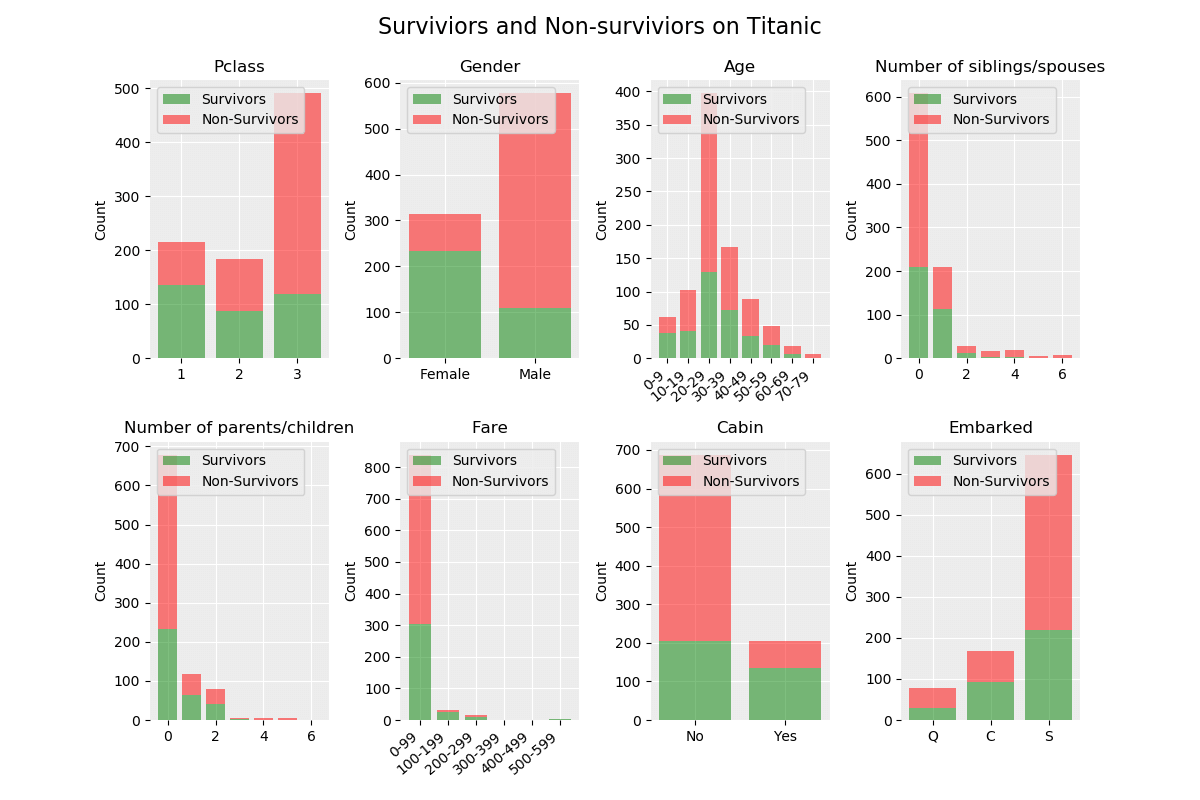
Baseline performance
The data set is not perfectly balanced as there is 549 non-survivors and 342 surviviors, a possible measure to get better results is to create a better balance in the data set. The probability to make a correct prediction of a non-survivor is 66.67 % (549/891) and our model must perform better than this.
Python module
The following module is used for training, evaluation and submission. I am using tree models which each has a lot of hyperparameters that can be adjusted. All of the project files is stored in annytab/decision_trees and the namespace for our common module is therefore annytab.decision_trees.
# Import libraries
import pandas
import joblib
import csv
import numpy as np
import sklearn.model_selection
import sklearn.tree
import sklearn.ensemble
import sklearn.metrics
import xgboost
import graphviz
import matplotlib.pyplot as plt
import annytab.decision_trees.common as common
# Train and evaluate
def train_and_evaluate():
# Load train data set (includes header values)
ds = pandas.read_csv('C:\\DATA\\Python-data\\titanic\\train.csv')
# Preprocess data
ids, ds = common.preprocess_data(ds)
# Slice data set in values and target (2D-array)
X = ds.values[:,1:9] # Data
Y = ds.values[:,0] # Survived
# Create models
models = []
models.append(('DecisionTree', sklearn.tree.DecisionTreeClassifier(criterion='gini', splitter='best', max_depth=None, min_samples_split=5, min_samples_leaf=1,
min_weight_fraction_leaf=0.0, max_features=None, random_state=None, max_leaf_nodes=None,
min_impurity_decrease=0.0, min_impurity_split=None, class_weight=None, presort=False)))
models.append(('RandomForest', sklearn.ensemble.RandomForestClassifier(n_estimators=100, criterion='gini', max_depth=None, min_samples_split=5,
min_samples_leaf=1, min_weight_fraction_leaf=0.0, max_features='auto',
max_leaf_nodes=None, min_impurity_decrease=0.0, min_impurity_split=None,
bootstrap=True, oob_score=False, n_jobs=None, random_state=None, verbose=0,
warm_start=False, class_weight=None)))
models.append(('XGBoost', xgboost.XGBClassifier(booster='gbtree', max_depth=6, min_child_weight=1, learning_rate=0.1, n_estimators=500, verbosity=0, objective='binary:logistic',
gamma=0, max_delta_step=0, subsample=1, colsample_bytree=1, colsample_bylevel=1, reg_alpha=0, reg_lambda=0,
scale_pos_weight=1, seed=0, missing=None)))
# Loop models
for name, model in models:
# Train the model on the whole data set
model.fit(X, Y)
# Save the model (Make sure that the folder exists)
joblib.dump(model, 'C:\\DATA\\Python-data\\titanic\\models\\' + name + '.jbl')
# Evaluate on training data
print('\n--- ' + name + ' ---')
print('\nTraining data')
predictions = model.predict(X)
accuracy = sklearn.metrics.accuracy_score(Y, predictions)
print('Accuracy: {0:.2f}'.format(accuracy * 100.0))
print('Classification Report:')
print(sklearn.metrics.classification_report(Y, predictions))
print('Confusion Matrix:')
print(sklearn.metrics.confusion_matrix(Y, predictions))
# Evaluate with 10-fold CV
print('\n10-fold CV')
predictions = sklearn.model_selection.cross_val_predict(model, X, Y, cv=10)
accuracy = sklearn.metrics.accuracy_score(Y, predictions)
print('Accuracy: {0:.2f}'.format(accuracy * 100.0))
print('Classification Report:')
print(sklearn.metrics.classification_report(Y, predictions))
print('Confusion Matrix:')
print(sklearn.metrics.confusion_matrix(Y, predictions))
# Predict and submit
def predict_and_submit():
# Load test data set (includes header values)
ds = pandas.read_csv('C:\\DATA\\Python-data\\titanic\\test.csv')
# Preprocess data
ids, ds = common.preprocess_data(ds)
# Slice data set in values (2D-array), test set does not have target values
X = ds.values[:,0:8] # Data
# Load the best models
model = joblib.load('C:\\DATA\\Python-data\\titanic\\models\\RandomForest.jbl')
# Make predictions
predictions = model.predict(X)
# Save predictions to a csv file
file = open('C:\\DATA\\Python-data\\titanic\\submission.csv', 'w', newline='')
writer = csv.writer(file, delimiter=',')
writer.writerow(('PassengerId', 'Survived'))
for i in range(len(predictions)):
writer.writerow((ids[i], predictions[i].astype(int)))
file.close()
# Print success
print('Successfully created submission.csv!')
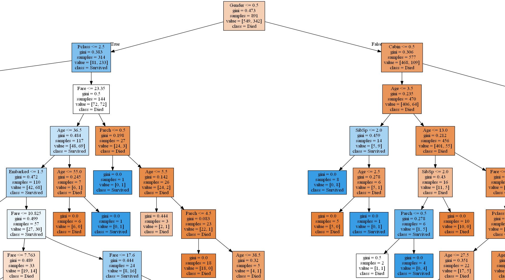
# Plot models
def plot_models():
# Load models
decision_tree_model = joblib.load('C:\\DATA\\Python-data\\titanic\\models\\DecisionTree.jbl')
random_forest_model = joblib.load('C:\\DATA\\Python-data\\titanic\\models\\RandomForest.jbl')
xgboost_model = joblib.load('C:\\DATA\\Python-data\\titanic\\models\\XGBoost.jbl')
# Names
feature_names = ['Pclass', 'Gender', 'Age', 'SibSp', 'Parch', 'Fare', 'Cabin', 'Embarked']
class_names = ['Died', 'Survived']
# Save decision tree model to an image
source = graphviz.Source(sklearn.tree.export_graphviz(decision_tree_model, out_file=None, feature_names=feature_names, class_names=class_names, filled=True))
source.render('C:\\DATA\\Python-data\\titanic\\plots\\decision-tree',format='png', view=False)
# Save random forest model to an image
source = graphviz.Source(sklearn.tree.export_graphviz(random_forest_model.estimators_[8], out_file=None, filled=True))
source.render('C:\\DATA\\Python-data\\titanic\\plots\\random-forest',format='png', view=False)
# Save xgboost model to an image
xgboost_model.get_booster().feature_names = feature_names
xgboost.plot_tree(xgboost_model, num_trees=0)
figure = plt.gcf()
figure.set_size_inches(100, 50)
plt.savefig('C:\\DATA\\Python-data\\titanic\\plots\\xgboost.png')
# The main entry point for this module
def main():
# Train and evaluate
#train_and_evaluate()
# Predict and submit
#predict_and_submit()
# Plot a model
plot_models()
# Tell python to run main method
if __name__ == "__main__": main()Training and evaluation
A for loop is used to train and evaluate models, each model is saved to a file. The output from the training and evaluation process is shown below.
--- DecisionTree ---

Training data
Accuracy: 94.84
Classification Report:
              precision    recall  f1-score   support

         0.0       0.94      0.98      0.96       549
         1.0       0.96      0.90      0.93       342

    accuracy                           0.95       891
   macro avg       0.95      0.94      0.94       891
weighted avg       0.95      0.95      0.95       891

Confusion Matrix:
[[536  13]
 [ 33 309]]

10-fold CV
Accuracy: 78.90
Classification Report:
              precision    recall  f1-score   support

         0.0       0.82      0.85      0.83       549
         1.0       0.74      0.70      0.72       342

    accuracy                           0.79       891
   macro avg       0.78      0.77      0.77       891
weighted avg       0.79      0.79      0.79       891

Confusion Matrix:
[[464  85]
 [103 239]]

--- RandomForest ---

Training data
Accuracy: 94.84
Classification Report:
              precision    recall  f1-score   support

         0.0       0.94      0.98      0.96       549
         1.0       0.97      0.90      0.93       342

    accuracy                           0.95       891
   macro avg       0.95      0.94      0.94       891
weighted avg       0.95      0.95      0.95       891

Confusion Matrix:
[[538  11]
 [ 35 307]]

10-fold CV
Accuracy: 82.27
Classification Report:
              precision    recall  f1-score   support

         0.0       0.84      0.88      0.86       549
         1.0       0.79      0.73      0.76       342

    accuracy                           0.82       891
   macro avg       0.82      0.81      0.81       891
weighted avg       0.82      0.82      0.82       891

Confusion Matrix:
[[483  66]
 [ 92 250]]

--- XGBoost ---

Training data
Accuracy: 98.20
Classification Report:
              precision    recall  f1-score   support

         0.0       0.98      0.99      0.99       549
         1.0       0.99      0.97      0.98       342

    accuracy                           0.98       891
   macro avg       0.98      0.98      0.98       891
weighted avg       0.98      0.98      0.98       891

Confusion Matrix:
[[544   5]
 [ 11 331]]

10-fold CV
Accuracy: 81.37
Classification Report:
              precision    recall  f1-score   support

         0.0       0.84      0.87      0.85       549
         1.0       0.77      0.73      0.75       342

    accuracy                           0.81       891
   macro avg       0.80      0.80      0.80       891
weighted avg       0.81      0.81      0.81       891

Confusion Matrix:
[[475  74]
 [ 92 250]]
Submission
I created a submission file by using the XGBoost model and uploaded the file to kaggle. My accuracy score was 0.73250, not much better than the baseline performance.
Plot trees
You will need to unpack or install Graphviz in order to plot models in Python. You also need to add a Path to the bin folder (C:\Program Files\Graphviz\bin) in environment variables. I load all the models and save plots as png:s, you can save them as pdf:s or other formats.